Benchmarking the Performance of R Code

To assess the performance of R code there's a great little package called microbenchmark.

install.packages('microbenchmark')
library(microbenchmark)

I was particularly interested in the performance increase of a shiny application that reads in a bunch of .csv data. To test the performance increase I ran the following code:

# For all *.csv files in "data" directory
csv.files <- list.files(path = "data", pattern = "*.csv", full.names = TRUE)

# How many csvs are there?
length(csv.files)
#[1] 13

# Benchmark
results <- microbenchmark(
  read.csv2.test = lapply(csv.files, read.csv2),
  read_csv.test  = lapply(csv.files, read_csv),
  times = 50)

So that's 50 iterations of reading 13 files, or 650 reads for each function. Now to have a look at the results:

> results
Unit: milliseconds
           expr       min        lq      mean    median        uq      max neval
 read.csv2.test 111.18612 118.28930 124.71949 123.38192 131.20016 144.3691    50
  read_csv.test  67.56371  71.28666  76.22763  74.19215  78.06555 105.8433    50

Not the most impressive gain from the readr package, where the documentation purports up to 10x faster reads, but still substantial and worth implementing. For a simple guide on UX and the implications of lag check out this stackexchange answer. And if you want even faster read/write operations have a look at data.table's fread() function.

Examine the Distribution of Evaluations #

The microbenchmark package includes a boxplot() function which is a really good idea to look at prior to implementing a particular change in your code base. Here's an example of a comparison between a custom function and the same function compiled using the compiler::cmpfun() function.

Here's the a print out of the results:

print(results)
## Unit: microseconds
##      expr    min      lq      mean  median      uq       max neval
##     plain 87.550 90.5355 227.71949 91.8995 94.5685 13308.578   100
##  compiled 87.254 90.9845  95.71651 92.4605 96.1630   194.724   100

If I only compared the mean of the two functions, then I would expect to get a considerable 58% speed increase.

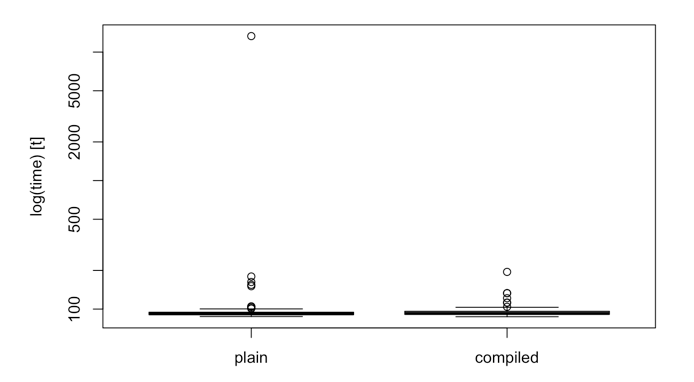
However, the boxplot of the results boxplot(results) quickly reveals an outlier in the 100 evaluations performed that heavily impacts the mean. In this case, the median actually shows a negligible difference between the function and the byte compiled function.

If you prefer a fancier looking plot, microbenchmark has included a ggplot2 based autoplot() function.

library(ggplot2)
autoplot(results)

When Should You Use Microbenchmarking? #

I use the microbenchmark package whenever I am concerned about speeding up an application. Old hands know the obligatory computer science mantra and the Knuth quote that must go along with this microbenchmarking blog post.

Make it work, make it right, make it fast.

-- Kent Beck

... premature optimization is the root of all evil...

-- Donald Knuth

Knuth goes on to say in his paper,'It is often a mistake to make a priori judgments about what parts of a program are really critical'. Which is why you should first profile your code to identify where your efforts are best spent.

Postscript - After a few nights of sleep I realised why the compiled vs. non-compiled functions had the distributions they did. Version 3.4 of R has Just-In-Time (JIT) compiling at level 3 by default. The function I was comparing contains a for loop. Therefore, the plots show the difference between the new JIT(3) speed of R vs pre-compiling your functions that contain for loops. The first run of the non-compiled function is not byte-compiled, however all subsequent runs are byte-compiled. Hence one outlier but otherwise very similar distributions.