Binary Classification in Python - Who's Going to Leave Next?
This post goes through a binary classification problem with Python's machine learning library scikit-learn.
Aim #
Create a model that predicts who is going to leave the organisation next. Commonly known as churn modelling.
To follow along, I breakdown each piece of the coding journey in this post. Alternatively, you can find a complete copy of the code on github. You'll need the following packages loaded:
import os
import pandas as pd
import numpy as np
import matplotlib.pyplot as plt
import seaborn as sns
from random import sample
from sklearn.linear_model import LogisticRegression
from sklearn import tree
from sklearn.ensemble import RandomForestClassifier
from sklearn.svm import SVC
from sklearn.neighbors import KNeighborsClassifier
from sklearn.naive_bayes import GaussianNB
from sklearn.cross_validation import cross_val_score
from sklearn import metrics
from IPython.display import Image
from pydotplus import graph_from_dot_data
The dataset for this exercise was originally found on kaggle. It's no longer available via Kaggle, so you can download a copy from my GitHub repo by running:
curl https://raw.githubusercontent.com/ucg8j/kaggle_HR/master/HR_comma_sep.csv >| HR_comma_sep.csvThen to read in the data:
# Set working directory
path = os.path.expanduser('~/Projects/kaggle_HR/')
os.chdir(path)
# Read in the data
df = pd.read_csv('HR_comma_sep.csv')
It contains data of 14,999 employees who are either in the organisation or have left, and 10 columns.
>>> df.shape
(14999, 10)
>>> df.columns.tolist()
['satisfaction_level',
 'last_evaluation',
 'number_project',
 'average_montly_hours',
 'time_spend_company',
 'Work_accident',
 'left',
 'promotion_last_5years',
 'sales',
 'salary']
We need to get some sense of how balanced our dataset is...
# Some basic stats on the target variable
print '# people left = {}'.format(len(df[df['left'] == 1]))
# people left = 3571

print '# people stayed = {}'.format(len(df[df['left'] == 0]))
# people stayed = 11428

print '% people left = {}%'.format(round(float(len(df[df['left'] == 1])) / len(df) * 100), 3)
# % people left = 24.0%
Knowing that 76% of the workforce will stay helps us not be excited by machine learning diagnostics that aren't much better than 76%. If I predicted that all staff would remain in the organisation, I would be 76% accurate!
I next check for missing values.
>>> df.apply(lambda x: sum(x.isnull()), axis=0)
satisfaction_level       0
last_evaluation          0
number_project           0
average_montly_hours     0
time_spend_company       0
Work_accident            0
left                     0
promotion_last_5years    0
sales                    0
salary                   0
No missing values, that's great. Next I look for correlations in the data.
# Correlation heatmap
correlation = df.corr()
plt.figure(figsize=(10, 10))
sns.heatmap(correlation, vmax=1, square=True, annot=True, cmap='cubehelix')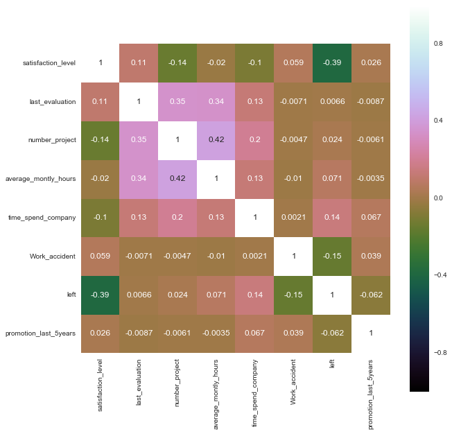
Unsurprisingly, satisfaction_level has the largest correlation with the decision to stay or leave. Next up, pairwise plots provide a lot information for one diagram.
# take a 5% sample as this is computationally expensive
df_sample = df.sample(frac=0.05)
# Pairwise plots
pplot = sns.pairplot(df_sample, hue="left")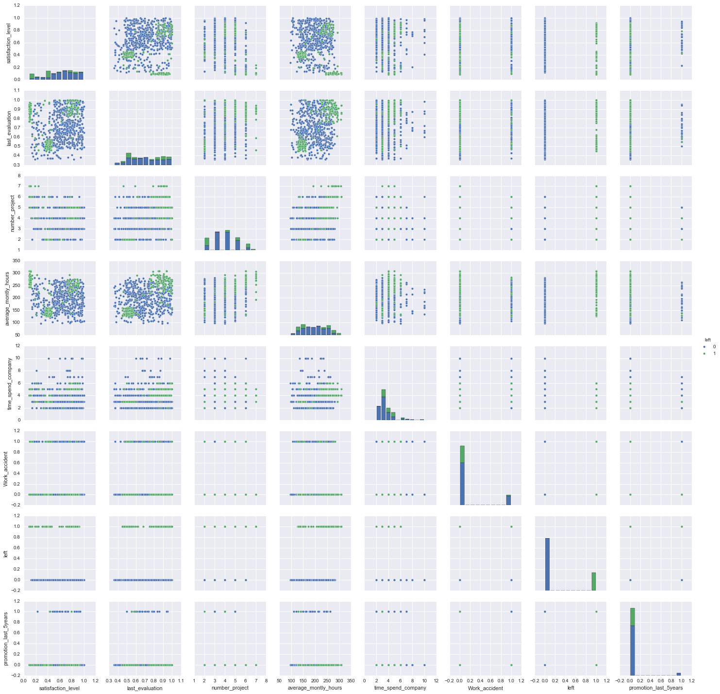
On the diagonal we can see the distribution of each variable, including the target variable of who has left (this visualises the balance). There are some interesting groupings of those who leave (Green dots) when looking at the plots of satisfaction_level by last_evaluation and by average_montly_hours - they look to be the same sub-populations. E.g. Low satisfaction but high evaluation and monthly hours, there's also a grouping of a high number of projects completed with low satisfaction levels by those who leave. Perhaps these are high performers that easily leave when they are not satisfied by their job. There are other interesting groupings so it's worth spending some time looking at this output examining these relationships. It's great to have these groupings, as our classifier should be able to differentiate between those who leave and those that remain. If there were no relationships revealed in this plot, we would face a very difficult problem and perhaps have to go back to examine what data we could collect to help predict the outcome.
Two variables were left out of the above plots, Salary and Sales. I need to deal with these separately prior to modelling, as our machine learning classifier will expect numbers to crunch rather than text.
>>> df.salary.unique()
array(['low', 'medium', 'high'], dtype=object)
>>> df.sales.unique()
array(['sales', 'accounting', 'hr', 'technical', 'support', 'management', 'IT', 'product_mng', 'marketing', 'RandD'], dtype=object)
Salary has 3 values low, medium and high. These factor variables have an order. I'm going to go use dummy encoding as a simple and common method to handle factor variables. The downsides to this is I am not handling the ordering and will introduce extra dimensions to the data (see Curse of dimensionality for why this is bad). Helmert, Forward/Backward differencing or Orthogonal encoding would probably be better.
As an aside... #
R makes factors really easy to handle. For example, let's say we have data with an unordered factor variable df$unordered.variable:
# Order a factor variable in R
df$ordered.var <- factor(df$unordered.var, levels = c('low', 'medium', 'high')
Dummy Encoding #
Dummy encoding, or one hot encoding, transforms categorical variables into a series of binary columns. Before I one hot encode the sales and salary I prepend the column names to the categories, that way I know later which column each new column came from. This helps particularly in cases where the columns use the same category names e.g. 'high' could apply to sales and salary.
# Prepend string prior to encoding
df['salary'] = '$_' + df['salary'].astype(str)
df['sales'] = 'sales_' + df['sales'].astype(str)

# Create 'salary' dummies and join
one_hot_salary = pd.get_dummies(df['salary'])
df = df.join(one_hot_salary)

# Create 'sales' dummies and join
one_hot_sales = pd.get_dummies(df['sales'])
df = df.join(one_hot_sales)
If we proceeded to modelling without dropping columns, we would run into the dummy variable trap. To illustrate what the dummy variable trap is, let's say that our data has a column for Gender in the form ['male','female','male','female'...]. If we use pd.get_dummies()
# Generate 'Gender' variable
Gender = np.random.choice(['male','female'], 4)
# Create DataFrame
df1 = pd.DataFrame(Gender, columns=['Gender'])
# One hot encode Gender
dummies = pd.get_dummies(df1['Gender'])
# Join dummies to 'df1'
df1 = df1.join(dummies)
print df1
   Gender  female  male
0    male       0     1
1  female       1     0
2    male       0     1
3  female       1     0
We can see that the dummy columns of female and male reflect the Gender column, a row with column Gender='male' has female=0 and male=1. In modelling, we are looking for independent variables to predict a dependent outcome. One of our dummy variables is completely dependent on the other (see Multicollinearity). We can naturally drop one of the dummy variables to avoid this trap whilst not losing any valuable information.
To avoid the dummy variable trap in the Kaggle HR dataset, I'm dropping the columns, sales_IT and low salary $_low.
# Drop unnecessary columns to avoid the dummy variable trap
df = df.drop(['salary', 'sales', '$_low', 'sales_IT'], axis=1)
Split Into Test and Training Sets #
Now to split the dataset up into our training, testing and optionally our validation sets. This is best done randomly to avoid having one subgroup of the data overrepresented in either our training or testing datasets, hence df.sample().
# Randomly, split the data into test/training/validation sets
train, test, validate = np.split(df.sample(frac=1), [int(.6*len(df)), int(.8*len(df))])
print train.shape, test.shape, validate.shape
# (8999, 20) (3000, 20) (3000, 20)
# Separate target and predictors
y_train = train['left']
x_train = train.drop(['left'], axis=1)
y_test = test['left']
x_test = test.drop(['left'], axis=1)
y_validate = validate['left']
x_validate = validate.drop(['left'], axis=1)
# Check the balance of the splits on y_
>>> y_test.mean()
0.23933333333333334
>>> y_train.mean()
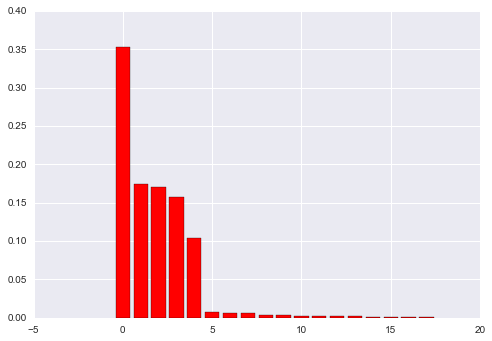
0.24091565729525502Feature importance can be ascertained from a random forest, alternatively Principal Components Analysis (PCA) can be used.
# Variable importance
rf = RandomForestClassifier()
rf.fit(x_train, y_train)
print "Features sorted by their score:"
print sorted(zip(map(lambda x: round(x, 4), rf.feature_importances_), x_train), reverse=True)
#[(0.3523, 'satisfaction_level'), (0.1738, 'time_spend_company'), (0.1705, 'number_project'), (0.158, 'average_montly_hours'), (0.1043, 'last_evaluation'), (0.0077, '$_high'), (0.0065, 'Work_accident'), (0.0059, '$_medium'), (0.0042, 'sales_technical'), (0.0034, 'sales_sales'), (0.0028, 'sales_support'), (0.0024, 'sales_hr'), (0.0023, 'sales_accounting'), (0.0019, 'sales_management'), (0.0014, 'sales_RandD'), (0.001, 'sales_product_mng'), (0.001, 'sales_marketing'), (0.0006, 'promotion_last_5years')]
A very rough plot of importances reveals that past the first 5 columns, we really don't get that much more variance explained by the additional columns.
From hereon in I'll only use the first 5 variables.
# Create variable lists and drop
all_vars = x_train.columns.tolist()
top_5_vars = ['satisfaction_level', 'number_project', 'time_spend_company', 'average_montly_hours', 'last_evaluation']
bottom_vars = [cols for cols in all_vars if cols not in top_5_vars]

# Drop less important variables leaving the top_5
x_train    = x_train.drop(bottom_vars, axis=1)
x_test     = x_test.drop(bottom_vars, axis=1)
x_validate = x_validate.drop(bottom_vars, axis=1)
Model Evaluation Basics #
The formula for accuracy is:
-
TP is the number of true positives
Predicted as leaving and they do
-
TN is the number of true negatives
Predicted as remaining and they do
-
FP is the number of false positives
Predicted as leaving, but they aren't - whoops!
-
FN is the number of false negatives
Predicted as remaining and they don't - eek!
As mentioned before, if we were aiming to predict those who remain (76%) then if we predicted 100%, we would have (0 + 11428) / 14999 or 76% accuracy. As the Accuracy Paradox wiki states precision and recall are probably more appropriate evaluation metrics. Here's a really quick definition of sensitivity (AKA recall), specificity and precision:
- Sensitivity/Recall -
TP / (TP + FN)how well the model recalls/identifies those that will leave. AKA the true positive rate. - Specificity -
TN / (TN + FP)how well the model identifies those that will stay. - Precision
TP / (TP + FP)how believable is the model? A low precision model will alarm you to those who are leaving that are actually staying. - F1 score
2 * (precision * recall)/(precision + recall)is the harmonic mean between precision and recall or the balance.
For this problem, we are perhaps most interested in knowing who is going to leave next. That way an organisation can respond with workforce planning and recruitment activities. Therefore, precision and recall will be the metrics we focus on.
Intuitively, precision is the ability of the classifier not to label as positive a sample that is negative, and recall is the ability of the classifier to find all the positive samples.
Source: scikit-learn
Modelling #
1. Logistic Regression #
Starting off with a very simple model, logistic regression.
# Instantiate
logit_model = LogisticRegression()
# Fit
logit_model = logit_model.fit(x_train, y_train)
# How accurate?
logit_model.score(x_train, y_train)
#0.7874

# How does it perform on the test dataset?

# Predictions on the test dataset
predicted = pd.DataFrame(logit_model.predict(x_test))
# Probabilities on the test dataset
probs = pd.DataFrame(logit_model.predict_proba(x_test))
print metrics.accuracy_score(y_test, predicted)
0.785
Now let's look at the confusion matrix and the metrics we care about.
>>> print metrics.confusion_matrix(y_test, predicted)
[[2100  182]
 [ 463  255]]
>>> print metrics.classification_report(y_test, predicted)
             precision    recall  f1-score   support

          0       0.82      0.92      0.87      2282
          1       0.58      0.36      0.44       718

avg / total       0.76      0.79      0.77      3000
Let's double check the classification_report. Focusing on those who will leave.
Precision = TP/(TP+FP) = 255/(255+182) = 0.58
Recall = TP/(TP+FN) = 255/(255+463) = 0.36
Perhaps we could optimise this model, however there are a range of models to test that may perform better out-of-the-box. I'll quickly run through a range of models...
2. Decision Tree #
Decision trees are highly interpretable and tend to perform well on classification problems.
# Instantiate with a max depth of 3
tree_model = tree.DecisionTreeClassifier(max_depth=3)
# Fit a decision tree
tree_model = tree_model.fit(x_train, y_train)
# Training accuracy
tree_model.score(x_train, y_train)

# Predictions/probs on the test dataset
predicted = pd.DataFrame(tree_model.predict(x_test))
probs = pd.DataFrame(tree_model.predict_proba(x_test))

# Store metrics
tree_accuracy = metrics.accuracy_score(y_test, predicted)
tree_roc_auc = metrics.roc_auc_score(y_test, probs[1])
tree_confus_matrix = metrics.confusion_matrix(y_test, predicted)
tree_classification_report = metrics.classification_report(y_test, predicted)
tree_precision = metrics.precision_score(y_test, predicted, pos_label=1)
tree_recall = metrics.recall_score(y_test, predicted, pos_label=1)
tree_f1 = metrics.f1_score(y_test, predicted, pos_label=1)

# evaluate the model using 10-fold cross-validation
tree_cv_scores = cross_val_score(tree.DecisionTreeClassifier(max_depth=3), x_test, y_test, scoring='precision', cv=10)

# output decision plot
dot_data = tree.export_graphviz(tree_model, out_file=None,
                     feature_names=x_test.columns.tolist(),
                     class_names=['remain', 'left'],
                     filled=True, rounded=True,
                     special_characters=True)
graph = graph_from_dot_data(dot_data)
graph.write_png("images/decision_tree.png")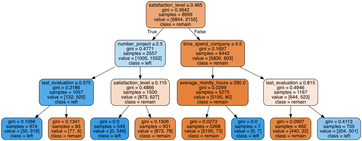
3. Random Forest #
# Instantiate
rf = RandomForestClassifier()
# Fit
rf_model = rf.fit(x_train, y_train)
# training accuracy 99.74%
rf_model.score(x_train, y_train)

# Predictions/probs on the test dataset
predicted = pd.DataFrame(rf_model.predict(x_test))
probs = pd.DataFrame(rf_model.predict_proba(x_test))

# Store metrics
rf_accuracy = metrics.accuracy_score(y_test, predicted)
rf_roc_auc = metrics.roc_auc_score(y_test, probs[1])
rf_confus_matrix = metrics.confusion_matrix(y_test, predicted)
rf_classification_report = metrics.classification_report(y_test, predicted)
rf_precision = metrics.precision_score(y_test, predicted, pos_label=1)
rf_recall = metrics.recall_score(y_test, predicted, pos_label=1)
rf_f1 = metrics.f1_score(y_test, predicted, pos_label=1)

# Evaluate the model using 10-fold cross-validation
rf_cv_scores = cross_val_score(RandomForestClassifier(), x_test, y_test, scoring='precision', cv=10)
rf_cv_mean = np.mean(rf_cv_scores)
This has performed possibly a little too well!
4. SUPPORT VECTOR MACHINE #
# Instantiate
svm_model = SVC(probability=True)
# Fit
svm_model = svm_model.fit(x_train, y_train)
# Accuracy
svm_model.score(x_train, y_train)

# Predictions/probs on the test dataset
predicted = pd.DataFrame(svm_model.predict(x_test))
probs = pd.DataFrame(svm_model.predict_proba(x_test))

# Store metrics
svm_accuracy = metrics.accuracy_score(y_test, predicted)
svm_roc_auc = metrics.roc_auc_score(y_test, probs[1])
svm_confus_matrix = metrics.confusion_matrix(y_test, predicted)
svm_classification_report = metrics.classification_report(y_test, predicted)
svm_precision = metrics.precision_score(y_test, predicted, pos_label=1)
svm_recall = metrics.recall_score(y_test, predicted, pos_label=1)
svm_f1 = metrics.f1_score(y_test, predicted, pos_label=1)

# Evaluate the model using 10-fold cross-validation
svm_cv_scores = cross_val_score(SVC(probability=True), x_test, y_test, scoring='precision', cv=10)
svm_cv_mean = np.mean(svm_cv_scores)
5. KNN #
# instantiate learning model (k = 3)
knn_model = KNeighborsClassifier(n_neighbors=3)
# fit the model
knn_model.fit(x_train, y_train)
# Accuracy
knn_model.score(x_train, y_train)

# Predictions/probs on the test dataset
predicted = pd.DataFrame(knn_model.predict(x_test))
probs = pd.DataFrame(knn_model.predict_proba(x_test))

# Store metrics
knn_accuracy = metrics.accuracy_score(y_test, predicted)
knn_roc_auc = metrics.roc_auc_score(y_test, probs[1])
knn_confus_matrix = metrics.confusion_matrix(y_test, predicted)
knn_classification_report = metrics.classification_report(y_test, predicted)
knn_precision = metrics.precision_score(y_test, predicted, pos_label=1)
knn_recall = metrics.recall_score(y_test, predicted, pos_label=1)
knn_f1 = metrics.f1_score(y_test, predicted, pos_label=1)

# Evaluate the model using 10-fold cross-validation
knn_cv_scores = cross_val_score(KNeighborsClassifier(n_neighbors=3), x_test, y_test, scoring='precision', cv=10)
knn_cv_mean = np.mean(knn_cv_scores)
6. TWO CLASS BAYES #
# Instantiate
bayes_model = GaussianNB()
# Fit the model
bayes_model.fit(x_train, y_train)
# Accuracy
bayes_model.score(x_train, y_train)

# Predictions/probs on the test dataset
predicted = pd.DataFrame(bayes_model.predict(x_test))
probs = pd.DataFrame(bayes_model.predict_proba(x_test))

# Store metrics
bayes_accuracy = metrics.accuracy_score(y_test, predicted)
bayes_roc_auc = metrics.roc_auc_score(y_test, probs[1])
bayes_confus_matrix = metrics.confusion_matrix(y_test, predicted)
bayes_classification_report = metrics.classification_report(y_test, predicted)
bayes_precision = metrics.precision_score(y_test, predicted, pos_label=1)
bayes_recall = metrics.recall_score(y_test, predicted, pos_label=1)
bayes_f1 = metrics.f1_score(y_test, predicted, pos_label=1)

# Evaluate the model using 10-fold cross-validation
bayes_cv_scores = cross_val_score(KNeighborsClassifier(n_neighbors=3), x_test, y_test, scoring='precision', cv=10)
bayes_cv_mean = np.mean(bayes_cv_scores)
Results #
# Model comparison
models = pd.DataFrame({
  'Model': ['Logistic', 'd.Tree', 'r.f.', 'SVM', 'kNN',  'Bayes'],
  'Accuracy' : [logit_accuracy, tree_accuracy, rf_accuracy, svm_accuracy, knn_accuracy, bayes_accuracy],
  'Precision': [logit_precision, tree_precision, rf_precision, svm_precision, knn_precision, bayes_precision],
  'recall' : [logit_recall, tree_recall, rf_recall, svm_recall, knn_recall, bayes_recall],
  'F1' : [logit_f1, tree_f1, rf_f1, svm_f1, knn_f1, bayes_f1],
  'cv_precision' : [logit_cv_mean, tree_cv_mean, rf_cv_mean, svm_cv_mean, knn_cv_mean, bayes_cv_mean]
})
# Print table and sort by test precision
models.sort_values(by='Precision', ascending=False)

   Model         F1 Accuracy Precision  cv_precision    recall
    r.f.   0.976812 0.989333  0.994100      0.988294  0.960114
  d.Tree   0.915088 0.959667  0.901798      0.899632  0.928775
     SVM   0.902098 0.953333  0.885989      0.863300  0.918803
     kNN   0.902959 0.953000  0.873502      0.831590  0.934473
   Bayes   0.530179 0.808000  0.620229      0.831590  0.462963
Logistic   0.327684 0.762000  0.483333      0.526624  0.247863
From the above results table, it is clear the Random Forest is the best model based on Accuracy, Precision and Recall metrics. The performance is so good, that I would be concerned about overfitting and a lack of generalisation to future periods of data. However, the classifier was evaluated with K-folds cross-validation (K=10) and also evaluated on the test dataset.
To use the trained model later, it's first best practice to re-train on the entire dataset to get the best trained model. Then save the pickle i.e. serialised model.
# Create x and y from all data
y = df['left']
x = df.drop(['left'], axis=1)

# Re-train model on all data
rf_model = rf.fit(x, y)

# Save model
import cPickle
with open('churn_classifier.pkl', 'wb') as fid:
    cPickle.dump(rf_model, fid)
The unabridged version of the above code can be found here on github.
Good Resources #
-
Cross Validated: How can machine learning models be used for survival analysis?
-
A very well written (human speak) blog on accuracy vs. recall & precision
-
Very simple explanation of ML evaluation metrics with nice visuals
-
High level overview of using transactional data for churn modelling
✍️ Want to suggest an edit? Raise a PR or an issue on Github